Non Linear Systems

Transfer functions can be used to describe any system in terms of its inputs and outputs

Generally we write this as $y=H(x)$ where $H(x)$ is the trasnfer function giving the output $y$ for an input $x$

Eg:

\[V_{out}=A \cdot V_{in} \\ H(x)=A \cdot x\]

$A$ is a constant and can be anything as long as it is not dependent on $x$

• A system is said to be linear if the ratio between input and output is the same regardless of the value of input.

• We can mathematically define whether a system is Linear or Non-Linear

If an input $x_1(t)$ produces the output $y_1(t)$ , and another input $x_2(t)$ produces the output $y_2(t)$ , then a system is linear if (and only if) an input of:

\[x(t)=Ax_1(t)+Bx_2(t)\\ =y(t)=Ay_1(t)+By_2(t)\]

Time-Invariant Systems

If a systems output is independent of time, it is time-invariant (in) If a systems output is dependent of time, it is time-variant

Non-Linear Systems

Most systems which are usually linear, will begin to exhibit non-linear behaviour when pushed too hard.

A non-linear transfer function will produce additional tones in the output which were not in the original input signal but are harmonically related to it

When analysing non-linear systems we distinguish between input signals based on whether the additional tones generated by them would be significant enough to cause noticeable non-linear behaviour in the output or not.

This is refered to as small-signal analysis and large-signal analysis

For small-signals the harmonic products are insignificant and the system acts linearly, there is a fixed ratio between the input and output signal.

For large-signals the harmonic products are significant and the system acts non-linearly, the output is no longer a fixed ratio of the input.

Non-Linear Circuit Analysis

The harmonic products generated in non-linear systems cause distortion of the output signal. Sometimes this is desirable, often it is not.

These tones were not in the original signal but are harmonically related to it.

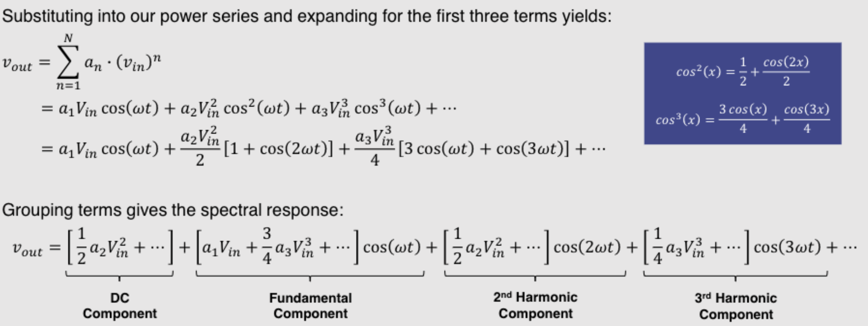
We can determine what these tones are by examining the system’s transfer function, this can be modelled using power series.

\[v_{out}=\sum_{n=1}^{N} a_n \cdot (v_{in})^n\]

Non-Linear Circuit Analysis (Signle Tone)

Consider a non-linear system excited by a large-signal input at a single frequency $v_{in}=v_{in} \cos(\omega t)$

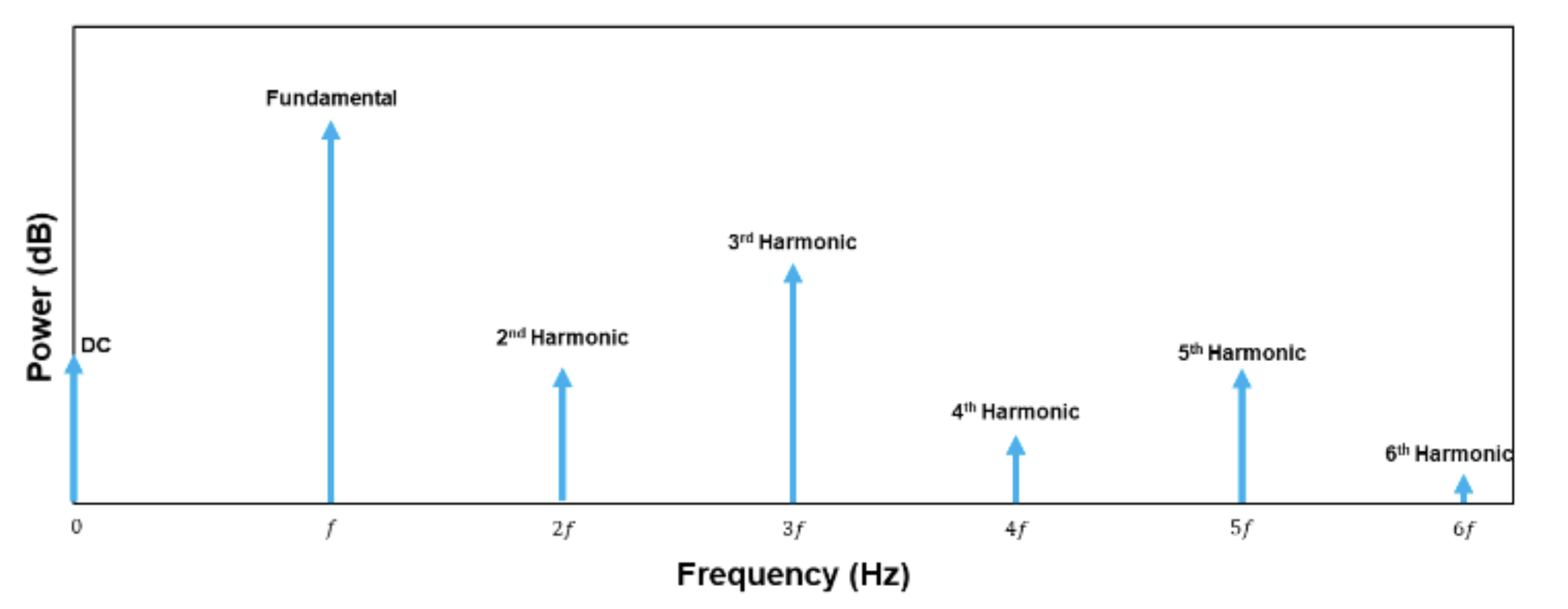
If we knew the magnitudes of these components and plotted the spectrum it would loosely resemble the graph below

For a single-tone input signal the additional products in the output will only be harmonic multiples of that frequency plus a small DC component

Non-Linear Circuit Analysis (Multiple Tone)

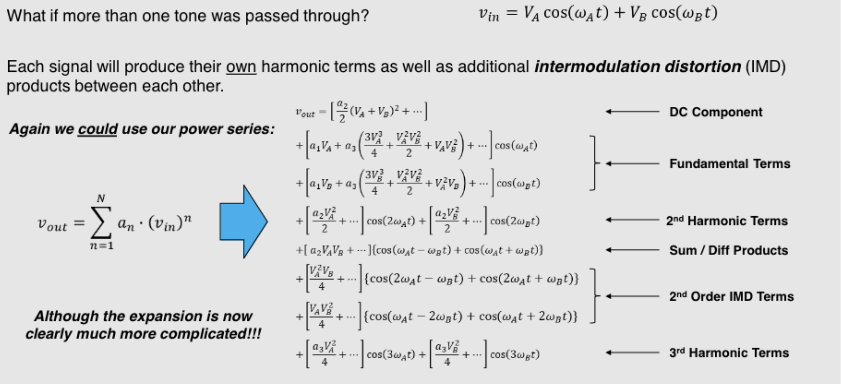
For a two-tone input signal the additional products in the output will be harmonics of both frequencies, plus their IMD products, plus a small DC component.

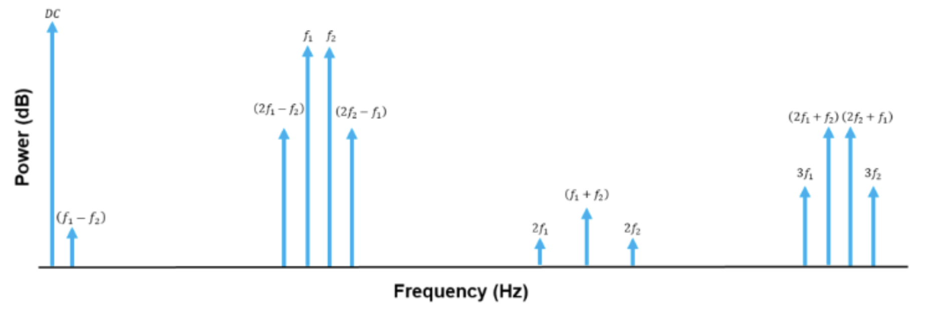
• For a single-tone; we would only have harmonics which are easily filtered off due to their even spacing
• For multiple-tones; intermodulation distortion (IMD) products appear all over the spectrum and are not so easily filtered off, this is referred to as Spectral Regrowth.

Total Harmonic Distortion

One method of characterising the linearity of a device (e.g. an amplifier) is by measuring its Total Harmonic Distortion (or THD). This is done by applying a spectrally pure sinewave to the device and observing the output spectrum.

Aa non-linear system excited in this way will produce additional harmonics in the output . (as well as a DC level shift). The degree to which this occurs gives a good measure of how linear the system can be expected to behave for a given operating condition.

THD is defined in terms of signal power however, since we might expect to measure the output spectrum in either amplitude or power, there are two equations we can use to calculate it:

SP measured in Power	SP measured in Voltage
:$100 \times \frac{\sqrt{P_2 + P_3 + P_n}}{P_1}=THD (\%)$:	:$100 \times \frac{\sqrt{V_2^2 + V_3^2 + V_n^2}}{V_1}=THD (\%)$:

$P_n$ is the power in watts, if measurement is in dB or dBm you must first convert. $V_n$ is the rms voltage, if measurement is peak voltage you must first convert. (Not Needed here as it will be cancel out $\sqrt{2}$)

Power Amplifiers

A Power Amplifier (or PA), is a circuit which provides finite positive gain at the frequency (or range of frequencies) of interest, their are different types of PA’s

• Low-Noise Amplifier (LNA)
• Wideband Amplifier (WBA)
• High-Power Amplifier (HPA)

An ideal power amplifier would be linear and have the transfer function

\[P_{out}=A \cdot P_in\]

Where $A$ is the gain of the amplifier $\therefore V_{out} is > V{in}$

Real power amplifiers are a good example of systems that become increasingly non-linear as they are pushed harder and harder by increasing the input signal power

The effect of these harmonics is a reduction in useful signal gain, and is referred to as gain compression.

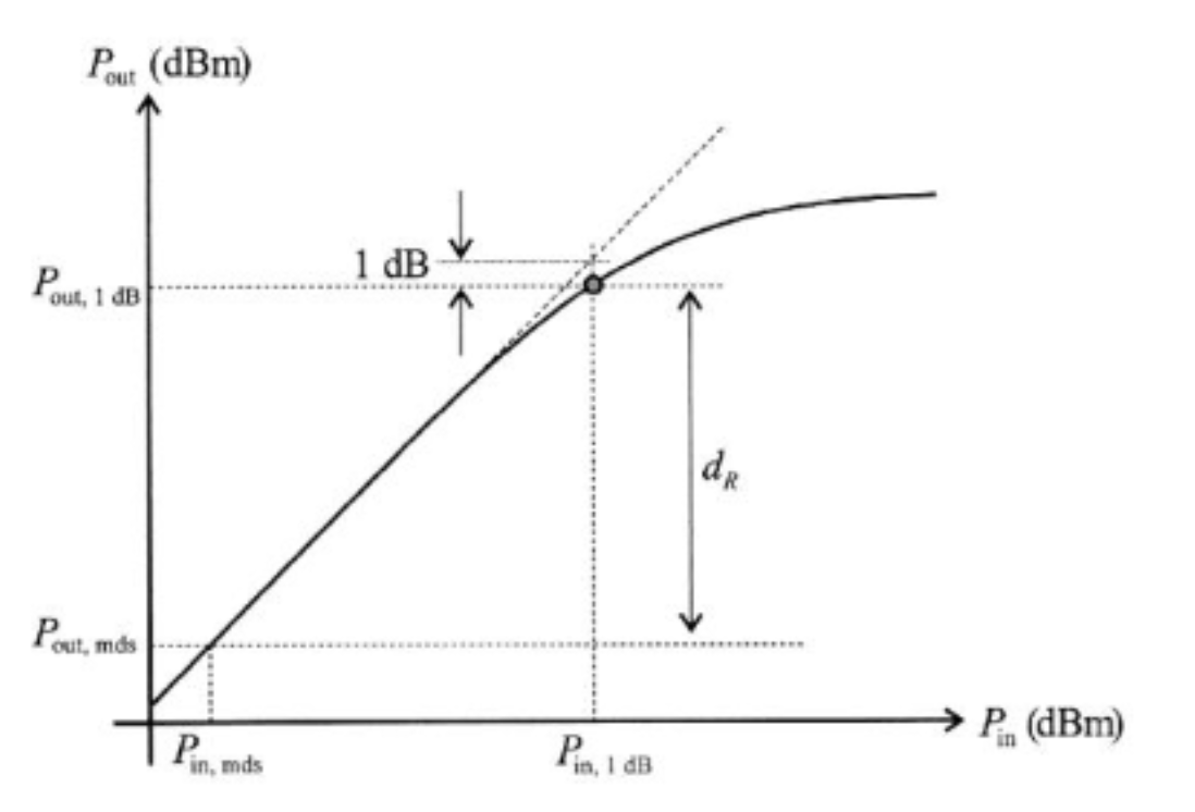
Dynamic Range and the 1dB Compression Point

The 1 dB compression point (often just referred to as the P1dB point) is defined for when the input power is large enough to cause a reduction in system gain (i.e. gain compression) of 1 dB (about 10%).

We define the dynamic range, $d_r$ of an amplifier as the range between the smallest and largest useful output power levels.

Smallest useful output power is given by the minimumdetectable signal, often determined by the noise floor

Largest useful output power is defined as the 1dB compression point, determined by the non-linear effects of the system

Dynamic Range can be calculated by: $d_r= P_{out,1db}-P_{out,mds}$

Amplifier Circuits

Power Amplifier circuits are classified based on the proportion of the input cycle that the amplifier circuit conducts in (a full cycle is $360^{\circ}$ degrees or $2\pi$ radians).

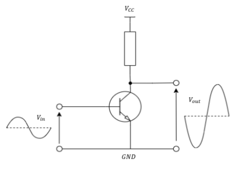
Class A Amplifiers

Class-A amplifiers conduct over the entire input cycle. In other words, the active device (normally a transistor)is always switched on.

• Simpler to implement than other classes as they only require one active device
• Tend to have fewer non-linear effects due to device always being ON and how it’s biased.
• Less efficient than other classes, theoretical max efficiency of Class A is 25%
• Because the device is always on, lifetime is reduced compared with other classes.

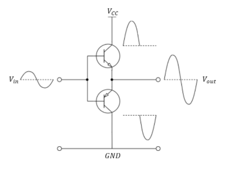
Class B Amplifiers

Class-B amplifiers conduct over half the input cycle (180°). The active device (a transistor) is only switched on half the time.

Since this would result in half the signal being lost, Class-B amplifiers are setup in pairs in a push-pull configuration.

• Higher efficiency compared to Class-A, theoretical maximum for Class-B is 78.5%
• Slight mismatching between the push-pull pair causes distortion as the devices switch on/off.This is called crossover distortion.

Operational Amplifiers

OpAmps are very versatile as they can be completely configured through external components to perform a number of functions:

• Inverting / Non-Inverting Amplifier
• Differential Amplifier
• Buffer Amplifier

The output of the inverting amplifier is given by: \(V_{out}=-\frac{R_f}{R_{in}}V_1\)

Where the gain is negative and given by the ratio between the input and feedback resistors $A=-\frac{R_f}{R_{in}}$

Additive Mixers

An Analogue Adder is a circuit which has two or more signal inputs, AC or DC, and a single output that is the arithmetic sum of the input voltages.

They are often called Additive Mixers or simply Adders

Mathematically described as:

\[V_{out} = V_1 + V _2 + V_n\]

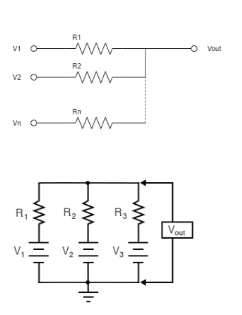
Passive Adder (Averaging Circuit)

The simplest form of adder is the passive adder which is a practical implementation of Millman’s Theorem:

\[V_out=\frac{\frac{V_1}{R_1}+\frac{V_2}{R_2}+\frac{V_n}{R_n}}{\frac{1}{R_1}+\frac{1}{R_2}+\frac{1}{R_n}}\]

If all resistances are the same value then the output voltage is the average of the inputs:

\[\frac{V_1 +V_2 +V_n}{n}\]

$n$ is number of inputs For this reason this circuit is often called a passive averaging circuit instead.

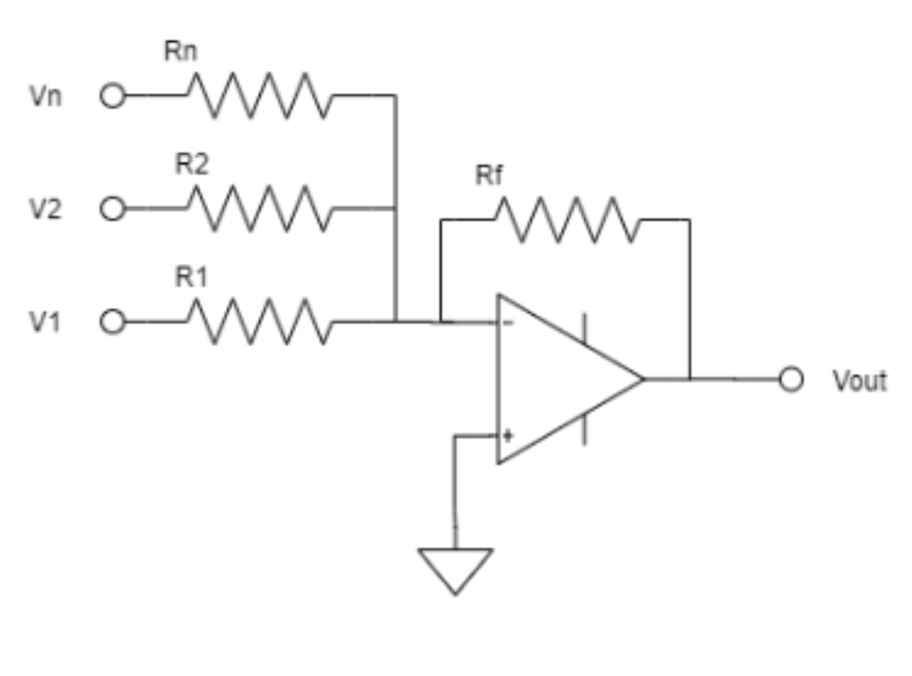
Active Adder (Summing Amplifier)

he main downside to the passive “adder” is that it is actually an averaging circuit, thus the output volttage will always be less than the sum of the inputs but still proportional

For a 2-input passive adder the output is given by the sum of the inputs divided by two:

$V_{out}=\frac{V_1 +V_2}{2}$

if we fed in to amplifier with gain 2 $V_{out}=2\cdot \frac{V_1 +V_2}{2}=V_1 +V_2$

Therefore this is a True adder and can be acheived by an op-amp or a transistor

This circuit is simply the passive averaging circuit fed into an inverting amplifier, Recalling the equation for an inverting OpAmp, our output is given by:

$V_{out}=-R_f(\frac{V_1}{R_1}+\frac{V_2}{R_2}+\frac{V_n}{R_n})$

if all the impedances are the same then:

$V_{out}=-\frac{R_f}{R_1}(V_1+V_2+V_n)$

here $\frac{R_f}{R_1}$ is the gain. Letting $R_f = R_1$ we get unity gain, andthe output is a true addition $V_{out}=-(V_1+V_2+V_n)$

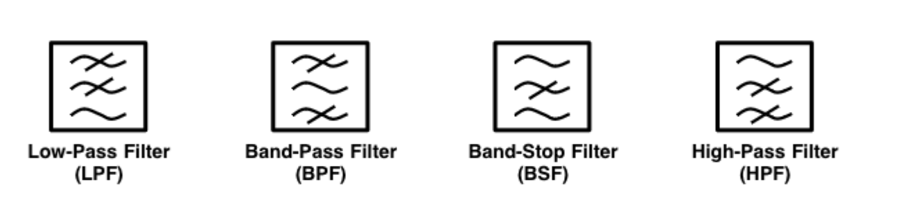
Filters

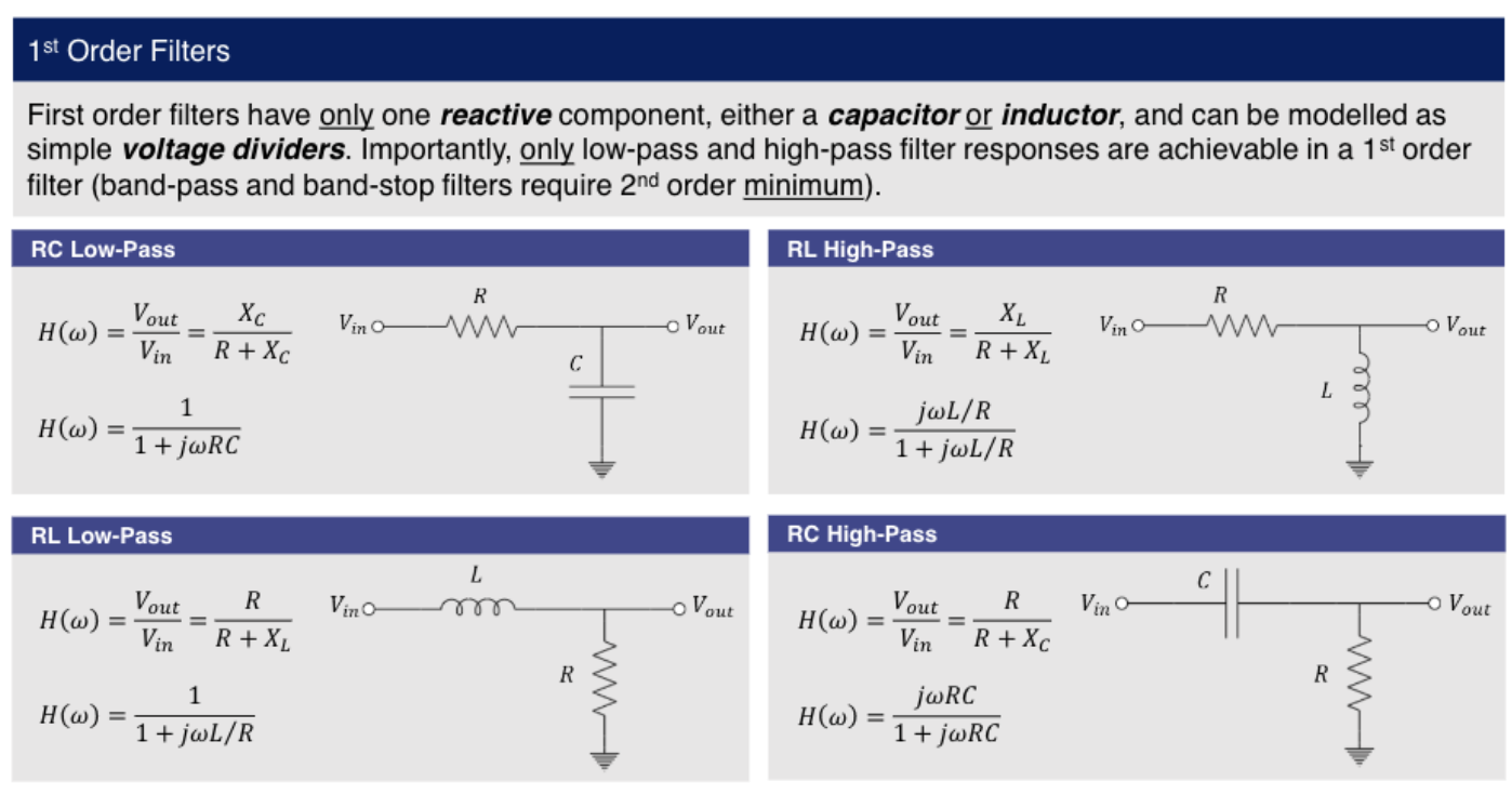
A Filter is a circuit which attenuates signals based on their frequency. Generally speaking a filter allows a defined range of frequencies to pass (passband) while rejecting others (stopband).

Where the passbad and stopband determines what type of filter it is Low-pass, High-pass, Band-pass & Band-stop

• The response of a filter is frequency dependant, and so reactive components (i.e. capacitors and inductors) have to be used.
• This means a filter’s transfer function will always be complex, by definition, and will modify both magnitude and phase
• Most filters are linear and so the output voltage can be found by multiplying the input by the magnitude of the complex transfer function:

\[V_{out}=abs(H(\omega)) \times v_{in}\]

Filter Classes

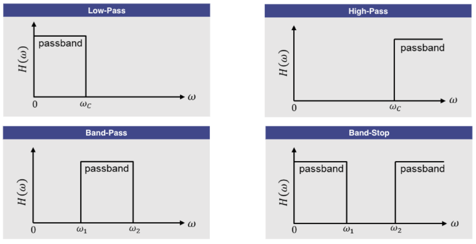
• Low-pass Filter: blocks signals with frequencies above cut-off frequency, and allows signals with frequencies below cut-off to pass.
• High-pass Filter: blocks signals with frequencies below cut-off frequency, and allows signals with frequencies above cut-off to pass.
• Band-pass Filter: blocks signals with frequencies outside the passband, and allows signals with frequencies inside the passband to pass.
• Band-stop Filter: blocks signals with frequencies inside the stopband, and allows signals with frequencies outside the stopband to pass.

Filter Repsonses

A perfect filter would only allow frequencies in its passband, and completely block those outside. In reality such a sharp cut-off is practically impossible, and real filters have a roll-off outside the pass-band determined by the filter’s order.

Unless the filter is an active one, there will be some small attenuation within the pass-band referred to as insertion loss (IL)

Additionally depending on the response type (Butterworth,Chebyshev, Bessel, etc.) there may also be some ripple in the passband

Filter Order

The roll-off of signal amplitudes outside of the pass-band is a key subject of interest in practical filter design. As mentioned, it can be shown that this roll-off rate can be related to something called the filters order.

The filter order is simply the number of reactive components it has. The simple RC circuit from before, was alow-pass filter (LPF); with only one reactive component (the capacitor), it is clearly a 1st Order LPF. Replacing the capacitor with an inductor would make it a 1st Order HPF.

The higher the filter order, the larger the gradient of roll-off response. For a 1st Order circuit the roll off is 20dB/decade (or 6dB/octave), for a 2nd order it is 40dB/decade (or 12dB/octave), and so on.

A Decade refers to increasing frequency by a power of 10: $f \times 10^n$

An Octave refers to increasing frequency by a power of 2: $f \times 2^n$